Polynomial Regression In Machine Learning

Polynomial regression is a type of regression analysis used in machine learning to model the relationship between the independent variable(s) and the dependent variable by fitting a polynomial equation to the data. It is particularly useful when the relationship between the variables is non-linear.

Polynomial Regression Equation

The general equation for polynomial regression of degree n is:

Y=a₀+a₁X +a₂X² +_ _ _ _ _+a_nXⁿ

By this equation, we are trying to find the best curve that fits our data.

• Y is the dependent variable we are trying to predict.
• X is the independent variable we are using to make predictions.
• a₀, a₁, a₂, _ _ _, a_n are the coefficients of the equation, which we need to find to get the best-fitting curve.

Example

Imagine you are trying to predict the price of a house (Y) based on its size (X). Instead of assuming that the relationship is a straight line, polynomial regression allows us to consider that maybe the relationship is not that simple.

So, our equation might look something like this:

House Price= a₀ + a₁ * Size + a₂ * Size²

In this equation:

a₀ is the base price of a house (maybe even if the house has no size).

a₁ tells us how much the price increases for every additional square foot.

a₂ captures any additional complexities in the relationship , like maybe larger houses have a higher price increase per square foot.

a₀, a₁, a_{2, _ _ _ _} a_n, the equation tries to fit the data points as closely as possible, giving us a curve that better represents the relationship between house size and price.

Steps of Polynomial Regression in Machine Learning

Step 1 Import Libraries

import numpy as np
import matplotlib.pyplot as plt
from sklearn.model_selection import train_test_split
from sklearn.linear_model import LinearRegression
from sklearn.preprocessing import PolynomialFeatures
from sklearn.metrics import mean_squared_error

Step 1 Prepare the Data

Sample data: House sizes (in square feet) and their corresponding prices

sizes = np.array([700, 800, 1000, 1200, 1500, 1800]).reshape(-1, 1)
prices = np.array([200000, 250000, 300000, 350000, 400000, 450000])

Step 3 Create Polynomial Features

poly_features = PolynomialFeatures(degree=2)
sizes_poly = poly_features.fit_transform(sizes)

Step 4 Split the Data into Training and Testing Sets

X_train, X_test, y_train, y_test = train_test_split(sizes_poly, prices, test_size=0.2, random_state=42)

Step 5 Train the Polynomial Regression Mode

model = LinearRegression()
model.fit(X_train, y_train)

Step 6 Evaluate the Model

train_pred = model.predict(X_train)
test_pred = model.predict(X_test)

print(f"Train MSE: {mean_squared_error(y_train, train_pred)}")
print(f"Test MSE: {mean_squared_error(y_test, test_pred)}")

Step 7 Make Predictions

size of the house we want to predict the price for

size_to_predict = np.array([[900]])  
size_to_predict_poly = poly_features.transform(size_to_predict)
predicted_price = model.predict(size_to_predict_poly)

In this

• We start by importing the necessary libraries.
• We create sample data for house sizes and prices.
• We use PolynomialFeatures from scikit-learn to create polynomial features of degree 2.
• We split the data into training and testing sets.
• We train a linear regression model using the polynomial features.
• We evaluate the model using Mean Squared Error (MSE).
• We make predictions for a new house size and print the predicted price.

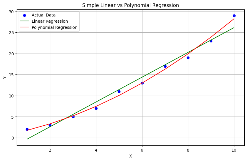
Graph of Polynomial Regression vs simple linear regression

In the above graph:

• The blue dots represent the actual data points.
• The green line represents the linear regression line.
• The red curve represents the polynomial regression curve.

You will notice that the linear regression line is straight, while the polynomial regression curve is more flexible and can capture more complex relationships in the data.