What is Regression In Machine Learning With a Example

Introduction

Regression is a statistical technique that is used to analyze the relationship between a dependent variable and one or more independent variables. As I have noted the objective is to find the most suitable function that characterizes the link between these variables. It seeks to find the best-fit model, which can be used to make predictions or conclusions. Let’s see What is Regression In Machine Learning With a Example.

In Machine Learning Regression is one of the supervised machine learning techniques.

A story that makes regression easy to understand

However imagine you’re a detective trying to crack the case of house prices. You know there are some key suspects: the size of the house and the number of bedrooms. Specifically these are your independent variables, the things you think might influence the price (the dependent variable), the big mystery you are trying to solve. Here’s where a regression model comes in. Generally it’s like a fancy interrogation technique. Overall you gather information on a bunch of houses – their size, bedrooms, and the selling price. The model then analyzes all this evidence and tries to establish a connection between the suspects (independent variables) and the crime scene (dependent variable).

Types of regression in machine learning

1. Linear Regression
2. Multiple Regression
3. Polynomial Regression
4. Logistic Regression
5. Ridge Regression and Lasso Regression

Linear Regression:
In linear regression, the relationship between the dependent variable and independent variable(s) is assumed to be linear. Generally it’s a straightforward approach suitable for situations where variables show a linear trend, approximated by a straight line.

class LinearRegression:
    def __init__(self, learning_rate=0.01, n_iterations=1000):
        self.learning_rate = learning_rate
        self.n_iterations = n_iterations
        self.weights = None
        self.bias = None

    def fit(self, X, y):
        n_samples, n_features = X.shape
        self.weights = np.zeros(n_features)
        self.bias = 0

        # Gradient descent
        for _ in range(self.n_iterations):
            y_predicted = np.dot(X, self.weights) + self.bias

            # Compute gradients
            dw = (1 / n_samples) * np.dot(X.T, (y_predicted - y))
            db = (1 / n_samples) * np.sum(y_predicted - y)

            # Update parameters
            self.weights -= self.learning_rate * dw
            self.bias -= self.learning_rate * db

    def predict(self, X):
        return np.dot(X, self.weights) + self.bias

model = LinearRegression(learning_rate=0.01, n_iterations=1000)
model.fit(X, y)

Types of Linear Regression in Machine Learning

• Simple Linear Regression
• Multiple Linear Regression

Simple Linear Regression:

Simple linear regression is a statistical technique that is used to find the relationship between a single independent variable (X) and a dependent variable (Y). It assumes a linear relationship between the two variables, which can be represented by a straight-line equation:

Y = β0 + β1X + ε

Where:

Y is the dependent variable (we want to predict),
X is the independent variable(used to make predictions),
β0 is the intercept of the line (the value of Y when X is 0),
β1 is the slope of the line (the change in Y for a one-unit change in X),
ε is the error term (the difference between the predicted and actual values of Y).
Here’s an example to illustrate simple linear regression:

So let’s say we want to predict the score a student will get on a test (Y) based on the number of hours they study (X). However we have data from several students showing their study hours and corresponding test scores. We can use simple linear regression to model this relationship.

Here’s a simplified dataset:

Therefore using simple linear regression, we can fit a line to this data that represents the relationship between study hours and test scores. Then after fitting the model, we can use it to predict test scores for new students based on the number of hours they study.

The regression equation might look like this:

Test Score = β0 + β1 * Hours Studied + ε

After fitting the model to the data, we might find that the equation is:

Test Score = 50 + 5 * Hours Studied + ε

Therefore this equation tells us that for every additional hour a student studies, we expect their test score to increase by 5 points, assuming all else remains constant. The intercept (β0) indicates that if a student studied 0 hours, we would expect their test score to be 50.

we can then use this equation to predict the test score of a student who studies, for example, 7 hours:

Test Score = 50 + 5 * 7 = 85

Multiple Linear Regression:

Overall multiple linear regression is a method to predict an outcome based on two or more input factors. So imagine you’re trying to predict a person’s weight based on their diet and exercise habits. Instead of just considering one factor like diet, multiple linear regression allows you to consider both diet and exercise together.

The equation for multiple linear regression looks like this:

y=b0+b1x1+b2x2+ ……..+bnxn

Here,

• y is the predicted outcome.
• b0 is the intercept, y value when all the input factors are zero.
• b1,b2,…… bn are the coefficients that represent how much each input factor affects the outcome.
• x1,x2,……,xn are the values of the input factors.

Multiple Regression:

Undoubtedly multiple regression builds upon linear regression by incorporating various independent variables to predict the dependent variable. It’s utilized when two or more independent variables influence the dependent variable.

Polynomial Regression:

Polynomial regression is employed when the relationship between the independent and dependent variables isn’t linear. Certainly this method allows for fitting a curve to the data, offering flexibility for capturing more complex relationships beyond straight lines.

Logistic Regression:

Logistic regression is specifically designed for situations where the dependent variable is binary (e.g., yes/no, 0/1). Undoubtedly it models the probability of the dependent variable belonging to a particular category, making it suitable for classification tasks.

Ridge Regression and Lasso Regressions

Ridge and Lasso regressions are regularization techniques applied to linear regression models to prevent overfitting and enhance performance. Ridge regression introduces a penalty term to the regression equation, while Lasso regression induces sparsity in the coefficient estimates, aiding in feature selection.

Polynomial Regression In Machine Learning

Specifically polynomial regression is a type of regression analysis used in machine learning to model the relationship between the independent variable(s) and the dependent variable by fitting a polynomial equation to the data. It is particularly useful when the relationship between the variables is non-linear.

Polynomial Regression Equation

The general equation for polynomial regression of degree n is:

Y=a₀+a₁X +a₂X² +_ _ _ _ _+a_nXⁿ

By this equation, we are trying to find the best curve that fits our data.

• Y is the dependent variable we are trying to predict.
• X is the independent variable we are using to make predictions.
• a₀, a₁, a₂, _ _ _, a_n are the coefficients of the equation, which we need to find to get the best-fitting curve.

Example

Certainly imagine you are trying to predict the price of a house (Y) based on its size (X). Instead of assuming that the relationship is a straight line, polynomial regression allows us to consider that maybe the relationship is not that simple.

So, our equation might look something like this:

House Price= a₀ + a₁ * Size + a₂ * Size²

In this equation:

a₀ is the base price of a house (maybe even if the house has no size).

a₁ tells us how much the price increases for every additional square foot.

a₂ captures any additional complexities in the relationship , like maybe larger houses have a higher price increase per square foot.

a₀, a₁, a_{2, _ _ _ _} a_n, the equation tries to fit the data points as closely as possible, giving us a curve that better represents the relationship between house size and price.

Steps of Polynomial Regression in Machine Learning

Step 1 Import Libraries

import numpy as np
import matplotlib.pyplot as plt
from sklearn.model_selection import train_test_split
from sklearn.linear_model import LinearRegression
from sklearn.preprocessing import PolynomialFeatures
from sklearn.metrics import mean_squared_error

Step 1 Prepare the Data

Sample data: House sizes (in square feet) and their corresponding prices

sizes = np.array([700, 800, 1000, 1200, 1500, 1800]).reshape(-1, 1)
prices = np.array([200000, 250000, 300000, 350000, 400000, 450000])

Step 3 Create Polynomial Features

poly_features = PolynomialFeatures(degree=2)
sizes_poly = poly_features.fit_transform(sizes)

Step 4 Split the Data into Training and Testing Sets

X_train, X_test, y_train, y_test = train_test_split(sizes_poly, prices, test_size=0.2, random_state=42)

Step 5 Train the Polynomial Regression Mode

model = LinearRegression()
model.fit(X_train, y_train)

Step 6 Evaluate the Model

train_pred = model.predict(X_train)
test_pred = model.predict(X_test)

print(f"Train MSE: {mean_squared_error(y_train, train_pred)}")
print(f"Test MSE: {mean_squared_error(y_test, test_pred)}")

Step 7 Make Predictions

size of the house we want to predict the price for

size_to_predict = np.array([[900]])  
size_to_predict_poly = poly_features.transform(size_to_predict)
predicted_price = model.predict(size_to_predict_poly)

In this

• We start by importing the necessary libraries.
• We create sample data for house sizes and prices.
• We use PolynomialFeatures from scikit-learn to create polynomial features of degree 2.
• We split the data into training and testing sets.
• We train a linear regression model using the polynomial features.
• We evaluate the model using Mean Squared Error (MSE).
• We make predictions for a new house size and print the predicted price.

Graph of Polynomial Regression vs simple linear regression

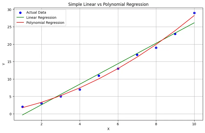
In the above graph:

• The blue dots represent the actual data points.
• The green line represents the linear regression line.
• The red curve represents the polynomial regression curve.

You will notice that the linear regression line is straight, while the polynomial regression curve is more flexible and can capture more complex relationships in the data.